The Stern-Gerlach experiment is not just an illustration; it is the physical thread that organizes the whole chapter. The analysis begins as classical mechanics of a magnetic moment in a field gradient, but the result of the experiment forces a discrete quantum description. The important point is that the apparatus translates a microscopic degree of freedom into spatially separated beams.
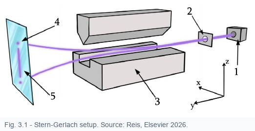
Silver atoms are evaporated in an oven, collimated into a narrow beam, and sent through a region where the magnetic field is inhomogeneous. The beam direction is taken as the \(y\)-axis; the useful separation happens in the \(z\)-direction. The glass plate at the end records where the atoms land.
The use of silver is physically convenient because the atom behaves like a system with one relevant valence electron. Modern atomic physics tells us that the orbital angular momentum of that electron in the ground configuration is zero, so the observed splitting is associated with spin rather than ordinary orbital motion.
A magnetic moment in a magnetic field has an interaction energy that depends on position when the field is not uniform. Taking the field as \(\mathbf B=(B_x,0,B_z)\), with the dominant variation along \(z\), the force component that matters for separation is obtained from the spatial derivative of the interaction:
With the simplifying assumptions used in the chapter, the cross derivatives vanish and the \(x\)-gradient is negligible. The result is the working Stern-Gerlach force law:
This equation is the classical gateway into the quantum problem: measuring the deflection is effectively measuring a component of the magnetic moment.
In the early interpretation, the atomic magnetic moment was related to orbital motion. A current loop of charge \(q\), speed \(v\), and orbital radius \(r\) gives
Since the orbital angular momentum is \(L=mvr\), this becomes
If the orbital angular momentum were continuously oriented, a continuous trace would be expected. If it were quantized, separated spots would appear. The experiment was historically read as evidence for angular-momentum quantization.
The observed discrete splitting survives, but its interpretation changes. Silver atoms have closed inner shells and one valence electron in an \(s\)-state. Because that orbital angular momentum is zero, the two-beam pattern is associated with an intrinsic degree of freedom: electron spin.
This is why the chapter later represents the relevant observable by a dimensionless spin operator \(\hat\sigma_u\), where \(u\) is the axis selected by the magnetic-field gradient. For a spin-1/2 system, the two possible dimensionless outcomes are
The apparatus therefore turns spin into a two-level measurement problem.
The book emphasizes that the experiment was first connected to the Bohr-era search for quantized angular momentum. Later developments, including Pauli's exclusion principle, Hund's rules, the proposal of spin by Uhlenbeck and Goudsmit, and Dirac's relativistic theory, clarified the interpretation. This history matters because it shows how experimental discreteness led to a new intrinsic quantum number.
| Level | Meaning |
|---|---|
| Classical expectation | A continuous distribution if magnetic moments can point in arbitrary directions. |
| Old quantum reading | Separated spots as evidence for angular-momentum quantization. |
| Modern reading | Two spots as evidence of a spin projection with two eigenvalues. |
The experiment already contains the postulates that the chapter will formalize. The incoming beam has a state; the magnet orientation defines the observable; the screen spots identify eigenvalues; the beam intensities give probabilities; and a selected outgoing beam becomes a prepared state for a later device.
This page is designed to support short guided exercises on: Inhomogeneous magnetic fields, magnetic moments, two spots and the interpretation of spin as a two-level observable.
- Use from this page: the definitions, physical setup, highlighted equations and conceptual links needed to start a first calculation or explanation.
- Keep in the book: complete derivations, extended historical discussion, worked solutions and the full textbook narrative remain in the original chapter and linked book resources.
- Good exercise balance: ask the student to identify assumptions, apply one relation, and interpret the result physically, without requiring material not introduced on this page.
Use these anchors to design compact exercises. The exercise should be answerable from this page plus standard algebra, while longer derivations, full worked examples and broader context should point back to the original book.
- Focus: Inhomogeneous magnetic fields, magnetic moments, two spots and the interpretation of spin as a two-level observable.
- Conceptual check: state what the main result says physically before using it algebraically.
- Equation: \[F_x=\frac{\partial}{\partial x}(\mu_xB_x+\mu_zB_z),\qquad F_y=0,\qquad F_z=\frac{\partial}{\partial z}(\mu_xB_x+\mu_zB_z).\]
- Equation: \[F_x\simeq0,\qquad F_y=0,\qquad F_z\simeq \mu_z\frac{\partial B_z}{\partial z}.\]
- Equation: \[\mu=IA=\frac{q}{2}vr.\]
- Boundary: use this page for setup and first-step reasoning; cite the book for longer derivations, complete experimental history or solved-problem detail.
- Typical task: derive, interpret, or apply the relation above to a simple case without introducing topics outside this page.