The QHO is described by a parabolic potential. The book introduces the dimensionless coordinate \(\xi=\alpha x\), obtains the Hermite differential equation, identifies its solutions, and then writes the normalized stationary eigenfunctions.
For \(V(x)=m\omega^2x^2/2\), the time-independent Schrödinger equation is
Box 4.1 introduces
Equation (4.2) then becomes
The book first considers the simpler particular case
whose solution is
It then writes
Substitution gives the equation for \(\chi(\xi)\):
This is the Hermite differential equation. The Gaussian factor ensures that \(\psi(x)\) decreases exponentially for large \(x\).
The solutions are \(\chi(\xi)=\chi_n(\xi)=A_nH_n(\xi)\), where \(A_n\) is a normalization constant and
are the Hermite polynomials. The first ones given in Box 4.2 are \(H_0(\xi)=1\), \(H_1(\xi)=2\xi\), \(H_2(\xi)=-2+4\xi^2\), and \(H_3(\xi)=-12\xi+8\xi^3\). Using the normalization condition, the book obtains
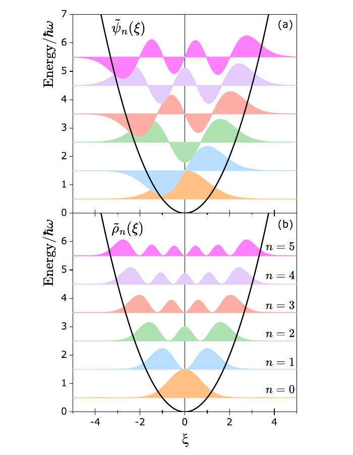
The figure represents Eq. (4.5). The number of minima in the probability-density curves, corresponding to nodes of the wave functions, is \(n\).
As discussed in the book after Figs. 4.1 and 4.2, the QHO probability density can extend beyond the classical turning points. This does not violate energy conservation: position and linear momentum cannot be measured simultaneously with absolute precision, so the classical notion of a turning point does not apply unchanged to the QHO.
This page is designed to support short guided exercises on: the QHO Schrödinger equation, the variables \(\alpha\), \(\xi\), and \(\epsilon\), the Hermite equation, Hermite polynomials, and the QHO wave functions.
- Use from this page: the definitions, physical setup, highlighted equations and conceptual links needed to start a first calculation or explanation.
- Keep in the book: complete derivations, extended historical discussion, worked solutions and the full textbook narrative remain in the original chapter and linked book resources.
- Good exercise balance: ask the student to identify assumptions, apply one relation, and interpret the result physically, without requiring material not introduced on this page.
Use these anchors to design compact exercises. The exercise should be answerable from this page plus standard algebra, while longer derivations, full worked examples and broader context should point back to the original book.
- Focus: the QHO Schrödinger equation, the variables \(\alpha\), \(\xi\), and \(\epsilon\), the Hermite equation, Hermite polynomials, and the QHO wave functions.
- Conceptual check: state what the main result says physically before using it algebraically.
- Equation: \[\hat H\psi(x)=\left[-\frac{\hbar^2}{2m}\frac{d^2}{dx^2}+\frac12m\omega^2x^2\right]\psi(x)=E\psi(x)\]
- Equation: \[\frac{d^2}{d\xi^2}\chi(\xi)-2\xi\frac{d}{d\xi}\chi(\xi)+(2\epsilon-1)\chi(\xi)=0\]
- Equation: \[\psi_n(x)=\left(\frac{m\omega}{\pi\hbar}\right)^{1/4}\frac{1}{\sqrt{2^n n!}}\exp\!\left(-\frac{m\omega}{2\hbar}x^2\right)H_n\!\left(\sqrt{\frac{m\omega}{\hbar}}x\right)\]
- Boundary: use this page for setup and first-step reasoning; cite the book for longer derivations, complete experimental history or solved-problem detail.
- Typical task: derive, interpret, or apply the relation above to a simple case without introducing topics outside this page.