After \(\hat L^2\) and \(\hat L_z\) have definite eigenvalues, the next question is what can still be said about the \(x\) and \(y\) components.
Writing \(\hat L_x\) and \(\hat L_y\) through \(\hat L_\pm\), the ladder action makes the relevant inner products proportional to \(\langle l,m|l,m\pm1\rangle\), which vanish.
This result is true for any allowed \(-l\le m\le +l\).
The next step is to calculate the quadratic operator. The terms \(\langle \hat L_+^2\rangle\) and \(\langle \hat L_-^2\rangle\) vanish by the same orthogonality argument.
The variance is the quadratic spread around the mean value. For any component, it is defined as
The standard deviation is the positive square root of the variance:
Using the quadratic averages above, the transverse variances follow as
The \(z\) component is precise in the state \(|l,m\rangle\), but the transverse components are not.
Even for the maximum projection \(m=l\), the transverse spread does not vanish:
Therefore the angular momentum is not absolutely aligned with the \(z\)-axis, even at maximum projection.
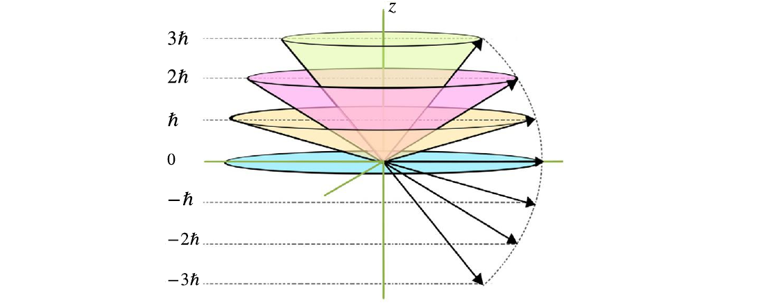
After a measurement of \(L_z\), the value of that component is precise. Since \(L_x\) and \(L_y\) retain finite variances, the angular momentum cannot be pictured as a classical vector pointing in one sharply defined direction.
The cone is a visualization aid: the magnitude \(\sqrt{l(l+1)}\hbar\) and the height \(m\hbar\) are fixed, while any position on the cone surface is equally probable.
This page supports guided exercises on: expectation values, transverse variances and the physical cone representation of angular momentum.
- Use from this page: the definitions, physical setup, highlighted equations and conceptual links needed for a compact calculation or explanation.
- Long-form material: complete proofs, long demonstrations, extended examples and the full exercise set remain in the textbook.
- Boundary: do not introduce results, notation or physical claims outside the sequence presented here and in Chapter 6.
Use these anchors only within the material introduced on this page.
- Focus: expectation values, transverse variances and the physical cone representation of angular momentum.
- Conceptual check: explain why \(\Delta L_z=0\) does not make \(\Delta L_x\) and \(\Delta L_y\) vanish.
- Key equation 1:
- Key equation 2:
- Key equation 3:
- Typical task: compute a variance for given \(l,m\) and interpret the cone picture.